Warning

Multi-node support is deprecated.

TimescaleDB v2.13 is the last release that includes multi-node support for PostgreSQL versions 13, 14, and 15.

Distributed hypertables are hypertables that span multiple nodes. With distributed hypertables, you can scale your data storage across multiple machines. The database can also parallelize some inserts and queries.

A distributed hypertable still acts as if it were a single table. You can work with one in the same way as working with a standard hypertable. To learn more about hypertables, see the hypertables section.

Certain nuances can affect distributed hypertable performance. This section explains how distributed hypertables work, and what you need to consider before adopting one.

Distributed hypertables are used with multi-node clusters. Each cluster has an access node and multiple data nodes. You connect to your database using the access node, and the data is stored on the data nodes. For more information about multi-node, see the multi-node section.

You create a distributed hypertable on your access node. Its chunks are stored on the data nodes. When you insert data or run a query, the access node communicates with the relevant data nodes and pushes down any processing if it can.

Distributed hypertables are always partitioned by time, just like standard hypertables. But unlike standard hypertables, distributed hypertables should also be partitioned by space. This allows you to balance inserts and queries between data nodes, similar to traditional sharding. Without space partitioning, all data in the same time range would write to the same chunk on a single node.

By default, Timescale creates as many space partitions as there are data nodes. You can change this number, but having too many space partitions degrades performance. It increases planning time for some queries, and leads to poorer balancing when mapping items to partitions.

Data is assigned to space partitions by hashing. Each hash bucket in the space dimension corresponds to a data node. One data node may hold many buckets, but each bucket may belong to only one node for each time interval.

When space partitioning is on, 2 dimensions are used to divide data into chunks: the time dimension and the space dimension. You can specify the number of partitions along the space dimension. Data is assigned to a partition by hashing its value on that dimension.

For example, say you use device_id as a space partitioning column. For each row, the value of the device_id column is hashed. Then the row is inserted into the correct partition for that hash value.

Expand image

Space partitioning dimensions can be open or closed. A closed dimension has a fixed number of partitions, and usually uses some hashing to match values to partitions. An open dimension does not have a fixed number of partitions, and usually has each chunk cover a certain range. In most cases the time dimension is open and the space dimension is closed.

If you use the create_hypertable command to create your hypertable, then the space dimension is open, and there is no way to adjust this. To create a hypertable with a closed space dimension, create the hypertable with only the time dimension first. Then use the add_dimension command to explicitly add an open device. If you set the range to 1, each device has its own chunks. This can help you work around some limitations of regular space dimensions, and is especially useful if you want to make some chunks readily available for exclusion.

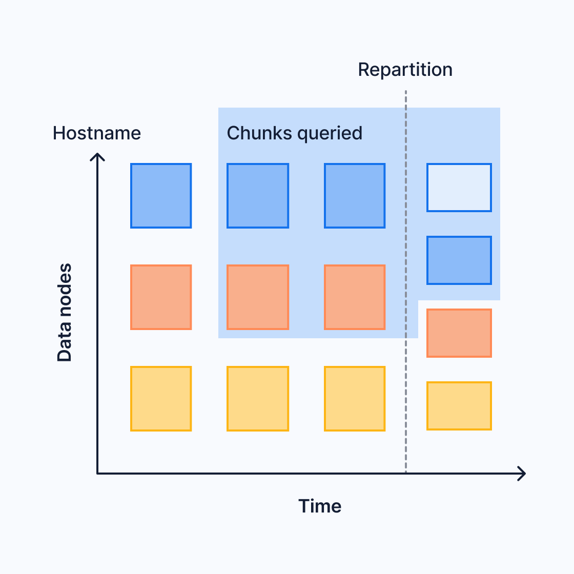
You can expand distributed hypertables by adding additional data nodes. If you now have fewer space partitions than data nodes, you need to increase the number of space partitions to make use of your new nodes. The new partitioning configuration only affects new chunks. In this diagram, an extra data node was added during the third time interval. The fourth time interval now includes four chunks, while the previous time intervals still include three:

Expand image

This can affect queries that span the two different partitioning configurations. For more information, see the section on limitations of query push down.

To replicate distributed hypertables at the chunk level, configure the hypertables to write each chunk to multiple data nodes. This native replication ensures that a distributed hypertable is protected against data node failures and provides an alternative to fully replicating each data node using streaming replication to provide high availability. Only the data nodes are replicated using this method. The access node is not replicated.

For more information about replication and high availability, see the multi-node HA section.

A distributed hypertable horizontally scales your data storage, so you're not limited by the storage of any single machine. It also increases performance for some queries.

Whether, and by how much, your performance increases depends on your query patterns and data partitioning. Performance increases when the access node can push down query processing to data nodes. For example, if you query with a GROUP BY clause, and the data is partitioned by the GROUP BY column, the data nodes can perform the processing and send only the final results to the access node.

If processing can't be done on the data nodes, the access node needs to pull in raw or partially processed data and do the processing locally. For more information, see the limitations of pushing down queries.

The access node can use a full or a partial method to push down queries. Computations that can be pushed down include sorts and groupings. Joins on data nodes aren't currently supported.

To see how a query is pushed down to a data node, use EXPLAIN VERBOSE to inspect the query plan and the remote SQL statement sent to each data node.

In the full push-down method, the access node offloads all computation to the data nodes. It receives final results from the data nodes and appends them. To fully push down an aggregate query, the GROUP BY clause must include either:

• All the partitioning columns or
• Only the first space-partitioning column

For example, say that you want to calculate the max temperature for each location:

SELECT location, max(temperature)
  FROM conditions
  GROUP BY location;

Copy

If location is your only space partition, each data node can compute the maximum on its own subset of the data.

In the partial push-down method, the access node offloads most of the computation to the data nodes. It receives partial results from the data nodes and calculates a final aggregate by combining the partials.

For example, say that you want to calculate the max temperature across all locations. Each data node computes a local maximum, and the access node computes the final result by computing the maximum of all the local maximums:

SELECT max(temperature) FROM conditions;

Copy

Distributed hypertables get improved performance when they can push down queries to the data nodes. But the query planner might not be able to push down every query. Or it might only be able to partially push down a query. This can occur for several reasons:

• You changed the partitioning configuration. For example, you added new data nodes and increased the number of space partitions to match. This can cause chunks for the same space value to be stored on different nodes. For instance, say you partition by device_id. You start with 3 partitions, and data for device_B is stored on node 3. You later increase to 4 partitions. New chunks for device_B are now stored on node 4. If you query across the repartitioning boundary, a final aggregate for device_B cannot be calculated on node 3 or node 4 alone. Partially processed data must be sent to the access node for final aggregation. The Timescale query planner dynamically detects such overlapping chunks and reverts to the appropriate partial aggregation plan. This means that you can add data nodes and repartition your data to achieve elasticity without worrying about query results. In some cases, your query could be slightly less performant, but this is rare and the affected chunks usually move quickly out of your retention window.
• The query includes non-immutable functions and expressions. The function cannot be pushed down to the data node, because by definition, it isn't guaranteed to have a consistent result across each node. An example non-immutable function is random(), which depends on the current seed.
• The query includes a user-defined function. The access node assumes the function doesn't exist on the data nodes, and doesn't push it down.

Timescale uses several optimizations to avoid these limitations, and push down as many queries as possible. For example, now() is a non-immutable function. The database converts it to a constant on the access node and pushes down the constant timestamp to the data nodes.

You can use distributed hypertables in the same database as standard hypertables and standard PostgreSQL tables. This mostly works the same way as having multiple standard tables, with a few differences. For example, if you JOIN a standard table and a distributed hypertable, the access node needs to fetch the raw data from the data nodes and perform the JOIN locally.